Sunday, January 31, 2016

Perl Basics

1.Perl is an scripting language
2. Practical extraction and report language
3. Basically used for text and data manipulation
4. It is an interpreted language
5. Doesn't need a special compiler to turn the scripts into working code
6. Do "which perl" to know the location of perl interpreter.
7. "perl filename" can be used for running the perl script.
Alternatively make "#! /usr/bin/perl" as the first line of your perl script.
8. Mostly .pl extension is associated with perl.
9. Give executable permission to the file before running :
Chmod + x hello.pl
10. Three main types of variables
Scalar, array and hash
$scalar, @array, %hash

11.  A singular variable is scalar and a plural variable is an array
12. Length of the variable name is not limited.
13. Variable names are case sensitive
14. Variable need not to be pre declared
15. No special character can be a part of variable name
16. Hash and array are used to hold scalar values
17. Normal arrays are indexed by number, and associative arrays by string.
18. Scalar variable can hold a string and a number
19. By default variables are global, unless defined otherwise
20. Use my keyword to declare variable as local

Tuesday, January 26, 2016

Data type in SV Part 4

1.Data types :
shortint, int, longint, bit , byte  //signed and 2 state (0 and 1)
logic, reg, time //unsigned and 4 state (0,1,X and Z)
integer  //signed and 4 state

2. user-defined datatype :
class, enumerations, struct, unions, typedef

3.Enumerations :  it is strongly typed and if we want to insert error. also if we don't initialize, then each one will have unique value .

methods : first, last, next, prev, name

4. Structured and Unions :
In structures we can have different data types which we can't have in array.

Diff between structures  and unions :
Same memory space is allocated for every members in UNIONS while in case of structures different mem space is allocated for each data members .

struct {int a; byte b; bit [7:0] c;} my_data ;

memory allocation for the above defined struct "my_data_struct". 


union { int a; byte b; bit [7:0] c; } my_data; 
Memory allocation for the above defined union "my_data_union". 


5. Typedef :
It lets us define our own identifiers
typedef bit[3:0] nibble ;
advantage :  reusable, shorter name, less error prone


Data type in SV - Part 3 : Arrays and Queues

Array :
Arrays hold a fixed number of equally-sized data elements. 
Individual elements are accessed by index using a consecutive range of integers. 
Some type of arrays allows to access individual elements using non consecutive values of any data types.
can be classified as fixed-sized/static arrays whose size cannot change once their declaration is done, or dynamic arrays, which can be resized. 

A.Fixed-Size Arrays : 
size is fixed

int low_high[0:15]   //16 ints 0 .... 15
int ary[16]   //16 ints 0 .... 15, in C style

Packed Array :
reg [0:10] ary  //Packed array, ary is a variable here ,
wire [31:0][1:0] ary  //2D Packed array, ary is a variable here ,

reg [31:0] ary1 [0:255] //unpacked array of 256 registers 
reg [31:0] ary1 [256] // register is packed 32 bit wide

 storage of an unpacked array : 


Array methods :
1. array querying method // $left. $right, $low, $high, $increment, $size
2. array locator method
2. array reduction method  //sum, product, or, and ,xor
3. array ordering method  // reverse, sort(in ascending order), rsort(in descending order), shuffle
4. array index querying            


B. Dynamic Array : 
1.It is an unpacked array
2. size can be set during run time .
3. this is done basically to avoid wasting of memory
4. It is used to deal with continuous collection of variables

integer ary1[] ; // declaration
ary1 = new [10] ; // allocation of memory

ary1 = new[10] ('{4,5,6,7,8,9})  // initialization ... here array elements are 4,5,6,7,8,9,9,0,0,0,0
ary1 = new[15] ary2   // resizing of ary1

if we want to copy the elements from different array

ary2 = new [100] ary1   //prev. ary1 elements will be reserved


C.Assosiative Arrays : when the size of collection is unknown or the data space is sparse, associatove array is better option,
it ensures faster access .

int ary [*]  ; //wildcard index (any integral type)
int ary[string];  //string index
int ary[class];   //class index
int ary[integer]; // integer ,,

here string, class or integer is called "keytype"
ary // array name
int // data type

No need to use new method for mem declaration ins case of associative array
methods : num/size, delete, exists, first, last, next, prev


4.Queues : 
1.variable size
2. ordered collection of homogeneous element
3. can be passed to tasks/functions as ref or non-ref arguments

int q[$] = {1,2,3} ;
int q[$]   // queue declaration
int e, pos ;
e = q[0]  // first element
e = q[$]  // last element

p = q //copy

Methods : size, insert, popfront, pop=back, push-front, push-back

Dynamic array of queues :
typedef int q[$] ;
q ary[]   ; // array of queues


Queues of queue :
typedef int q[$] ;
q p[$] ;


COMPARISON OF ARRAYS   // from testbench.in

Static Array 
Size should be known at compilation time. 
Time require to access any element is less. 
if not all elements used by the application, then memory is wasted.
Not good for sparse memory or when the size changes. 
Good for contagious data. 


Associative Array 
No need of size information at compile time. 
Time require to access an element increases with size of the array.
Compact memory usage for sparse arrays. 
User don't need to keep track of size. It is automatically resized. 
Good inbuilt methods for Manipulating and analyzing the content. 

Dynamic Array
No need of size information at compile time. 
To set the size or resize, the size should be provided at runtime. 
Performance to access elements is same as Static arrays. 
Good for contagious data. 
Memory usage is very good, as the size can be changed dynamically. 


Queues 
No need of size information at compile time. 
Performance to access elements is same as Static arrays. 
User doesn't need to provide size information to change the size. It is automatically resized. 
Rich set of inbuilt methods for Manipulating and analyzing the content. 
Useful in self-checking modules. Very easy to work with out of order transactions. 
Inbuilt methods for sum of elements, sorting all the elements. 
Searching for elements is very easy even with complex expressions.
Useful to model FIFO or LIFO. 


If your code accidently tries to read from an out-of-bounds address, System-
Verilog will return the default value for the array element type. That just means
that an array of 4-state types, such as logic , will return X’s, whereas an array of
2-state types, such as int or bit , will return 0. This applies for all array types –
fi xed, dynamic, associative, or queue, and also if your address has an X or Z. An
undriven net is Z.If your code accidently tries to read from an out-of-bounds address, System-
Verilog will return the default value for the array element type. That just means
that an array of 4-state types, such as logic , will return X’s, whereas an array of
2-state types, such as int or bit , will return 0. This applies for all array types –
fi xed, dynamic, associative, or queue, and also if your address has an X or Z. An
undriven net is Z.


Data type in SV : part 2 (The logic type )

The Logic type :

1. In verilog we use two reg and wire for driving a port and connecting a block respectively .

2.Wire is used to connect gates or modules and are physical wire in a circuit and it must be driven by a continues assignment statements.

3.“Reg” in Verilog is a data object that holds its value from one procedural statement to next. When we say "reg (register datatype)" it does not mean the register in the hardware or a physical register in circuit. This is the common mistake or assumption mostly engineers thinks while learning Verilog.

4.In SV reg and wire are replaced with a single data type that is logic.
5.It is 4 state (1, 0, X, Z) System Verilog data type.

6.“logic” signal can be used anywhere a “net” used but there is one exception to this, you can not drive logic variable from multiple driver. Logic type can only have a single drive,

7. This means we can declare all signal as logic to find if is there any multiple driver issue. Because in this case you should be able to see compilation issue if there is any multiple driver by declaring all signal with type “logic”.
8. The signal you would like to have multiple drivers shall be declared as net type such as “wire” or “tri”

Data types in SV : Part 1

#System Verilog introduces new data types with the following benefits.
• Two-state: better performance, reduced memory usage
• Queues, dynamic and associative arrays: reduced memory usage, built-in support
for searching and sorting
• Classes and structures: support for abstract data structures
• Unions and packed structures: allow multiple views of the same data
• Strings: built-in string support
• Enumerated types: code is easier to write and understand

#Verilog-1995 has two basic data types:
1. variables and nets, both which hold 4-state , values: 0, 1, Z, and X.
2. RTL code uses variables to store combinational and sequential
values.
3. Variables can be unsigned single or multi-bit ( reg [7:0] m ), signed
32-bit variables ( integer ), unsigned 64-bit variables ( time ), and floating point
numbers ( real ).
4. Variables can be grouped together into arrays that have a fixed
size.
5. A net is used to connect parts of a design such as gate primitives and module
instances.
6. Lastly, all storage is static, meaning that all variables are alive for the entire simulation and routines cannot use a stack to hold arguments and local values. 7. #Verilog-2001 allows you to switch between static and dynamic storage, such as stacks.
# SystemVerilog adds many new data types to help both hardware designers and
verification engineers.

Note : int i ; //  2 state , 32 bit signed integer
Signed variables can cause unexpected
results with randomization, will discuss more about it later


Sunday, January 24, 2016

Fork Join

The fork...join construct enables the creation of concurrent processes from each of its parallel statements.
SystemVerilog provides following version's of fork-join.

1.fork ... join //(join all)
2.fork ... join_none
3.fork ... join_any

4.disable fork ; //yes we need to use ; here , part of syntax
5.wait fork ; //yes we need to use ; here , part of syntax

//example 1
fork
p1 //suppose it takes 2ns
p2 //suppose it takes 3ns
join // p1 and p2 are parallel here
p3 // p3 will be executed only after finishing the process p1 and  p2, means only after the time 3ns


//example 2
fork
begin
p1 //suppose it takes 2ns
p2 //suppose it takes 3ns
end
join // p1 and p2 are parallel here
p3 // p3 will be executed only after finishing the process p1 and  p2, means only after the time 5ns, using begin end making it sequential


//example 3
fork
p1 //suppose it takes 2ns
p2 //suppose it takes 3ns
join_any // p1 and p2 are parallel here
p3 // p3 will be executed only after finishing the any of the process, whatever takes less time means only after the time 3ns(p2)


//example 4
fork
begin
p1 //suppose it takes 2ns
p2 //suppose it takes 3ns
end
join_any // p1 and p2 are parallel here
p3 // p3 will be executed only after finishing the process p1 and  p2, means only after the time 5ns, using begin end making it sequential


If we want to run all the process parallel and we want to wait for the completion of all the threads before any new step to be executed
use wait fork like this
//example 5
foreach[i]  //i is an 8 bit array which will give 8 values , so the loop will be executed 8 times
begin
fork
begin  // this begin will make the p1 and p2 sequential otherwise p1 and p2 will execute simultaneously as soon as the foreach loop starts
p1 //process p1 or thread p1
p2 //process p2 or thread p2
end
join_none
end
wait fork ;


//example 6
fork
p1
p2
join_any
disable fork;

in join_any , if one process is complete, and it is out form fork , but the other process will be running in the background and if we dont need it, we use disable fork .


Note from : (http://stackoverflow.com/questions/14287446/proper-use-of-disable-fork-in-systemverilog)
disable fork" kills not only the processes launched by your fork...join_any, but also any other processes that are descendants of the same process that executes the disable-fork. If you have launched any other processes (using, for example, fork...join_none) earlier in the life of this process, then those other processes will be killed too.
You can rather easily protect against this by causing your fork...join_any, and its later disable-fork, to run in a new child process of its own. This limits the effect of your disable-fork so that it can affect only the newly launched processes that you care about, and is guaranteed to have no other unwanted effects.
Do this by enclosing the whole mess in "fork begin...end join" like this:
fork begin // isolate the following code as a single child process
  fork  // launch the processes you wish to manage
    apply_input();
    update_status();
    verify_status();
  join_any // kill off the *_status threads when apply_input terminates
  disable fork;
end join // end of child process isolation
This is a well-known issue with fork...join_any and fork...join_none. It's been discussed recently on Verification Guild forum, and is described in sections #79 and #80 of the Sutherland and Mills book "Verilog and SystemVerilog Gotchas".
Putting "fork begin" and "end join" on single lines is unusual, but I like it as a way to make it very obvious that I'm synchronously forking exactly one child process. Normally that would be a useless thing to do, but in this situation it's essential.

Next interesting scenario: you have exited fork loop by join_none or join_any and after some steps, you want to kill just one thread (out of many). The solution, have named begin end block and call "disable ". (For example, in the last example if you want to kill only the 2nd thread after exiting the loop via join_any/join_none, then add "disable Second_thread;" at the point where you want to disable the second thread


General Note 1 : While learning SV or UVM, we also need to learn the appropriate term and the actual meaning of that word, so that we can co-relate it better.

Saturday, September 26, 2015

Clocking block in system verilog

1. Clocking blocks have been introduced in SystemVerilog to address the problem of specifying the timing and synchronisation requirements of a design in a testbench.

2. A clocking block is a set of signals synchronised on a particular clock.

3. It basically separates the time related details from the structural, functional and procedural elements of a testbench.

4. It helps the designer develop test benches in terms of transactions and cycles. Clocking blocks can only be declared inside a module, interface or program.
First Example
Here is a simple example to illustrate how SystemVerilog’s clocking construct works. Consider a loadable, up/down binary counter:
module COUNTER (input Clock, Reset, Enable, Load, UpDn,
                input [7:0] Data, output reg[7:0] Q);
  always @(posedge Clock or posedge Reset)
    if (Reset)
      Q <= 0;
    else
      if (Enable)
        if (Load)
          Q <= Data;
        else
          if (UpDn)
            Q <= Q + 1;
          else
            Q <= Q - 1;
endmodule

The testbench to test this counter, without using the clocking construct, might look like this:
module Test_Counter;
  timeunit 1ns;

  reg Clock = 0, Reset, Enable, Load, UpDn;

  reg [7:0] Data;
  wire [7:0] Q;
  reg OK;

  // Clock generator
  always
  begin
    #5 Clock = 1;
    #5 Clock = 0;
  end

  // Test stimulus
  initial
  begin
    Enable = 0;
    Load = 0;
    UpDn = 1;
    Reset = 1;
    #10; // Should be reset
    Reset = 0;
    #10; // Should do nothing - not enabled
    Enable = 1;    #20; // Should count up to 2
    UpDn = 0;
    #40; // Should count downto 254
    UpDn = 1;

    // etc. ...
  end

  // Instance the device-under-test
  COUNTER G1 (Clock, Reset, Enable, Load, UpDn, Data, Q);

  // Check the results
  initial
  begin
    OK = 1;
    #9;
    if (Q !== 8'b00000000)
      OK = 0;
    #10;
    if (Q !== 8'b00000000)
      OK = 0;
    #20;
    if (Q !== 8'b00000010)
      OK = 0;
    #40;
    if (Q !== 8'b11111110)
      OK = 0;
    // etc. ...
  end
endmodule
The testbench using clocking will look like this:
module Test_Counter_w_clocking;
  timeunit 1ns;

  reg Clock = 0, Reset, Enable, Load, UpDn;
  reg [7:0] Data;
  wire [7:0] Q;

  // Clock generator
  always
  begin
    #5 Clock = 1;
    #5 Clock = 0;
  end

  // Test program
  program test_counter;
    // SystemVerilog "clocking block"
    // Clocking outputs are DUT inputs and vice versa
    clocking cb_counter @(posedge Clock);
      default input #1step output #4;
      output negedge Reset;
      output Enable, Load, UpDn, Data;
      input Q;
    endclocking

    // Apply the test stimulus
    initial begin

      // Set all inputs at the beginning   
      Enable = 0;           
      Load = 0;
      UpDn = 1;
      Reset = 1;

      // Will be applied on negedge of clock!
      ##1 cb_counter.Reset  <= 0;
      // Will be applied 4ns after the clock!
      ##1 cb_counter.Enable <= 1;
      ##2 cb_counter.UpDn   <= 0;
      ##4 cb_counter.UpDn   <= 1;
      // etc. ...     
    end

    // Check the results - could combine with stimulus block
    initial begin
      ##1  
      // Sampled 1ps (or whatever the precision is) before posedge clock
      ##1 assert (cb_counter.Q == 8'b00000000);
      ##1 assert (cb_counter.Q == 8'b00000000);
      ##2 assert (cb_counter.Q == 8'b00000010);
      ##4 assert (cb_counter.Q == 8'b11111110);
      // etc. ...     
     end

    // Simulation stops automatically when both initials have been completed

  endprogram

  // Instance the counter
  COUNTER G1 (Clock, Reset, Enable, Load, UpDn, Data, Q);

  // Instance the test program - not required, because program will be
  // instanced implicitly.
  // test_COUNTER T1 ();
endmodule
There are a few important things to note: the testbench is implemented as a module, with a nested program that contains the clocking block (the full explanation of the advantages of implementing a testbench using a program can be found in the Program article). Program blocks can be nested within modules or interfaces. This way multiple co-operating programs can share variables local to the scope. Nested programs with no ports or top-level programs that are not explicitly instantiated are implicitly instantiated once. Implicitly instantiated programs have the same instance and declaration name.
The clocking construct is both the declaration and the instance of that declaration. Note that the signal directions in the clocking block within the testbench are with respect to the testbench. So Q is an output of COUNTER, but a clocking input. Note also that widths are not declared in the clocking block, just the directions.
The signals in the clocking block cb_counter are synchronised on the posedge of Clock, and by default all signals have a 4ns output (drive) skew and a #1step input (sample) skew. The skew determines how many time units away from the clock event a signal is to be sampled or driven. Input skews are implicitly negative (i.e. they always refer to a time before the clock), whereas output skews always refer to a time after the clock.
An input skew of #1step indicates that the value read by the active edge of the clock is always the last value of the signal immediately before the corresponding clock edge. A step is the time precision.
The ## operator is used in the testbench to delay execution by a specified number of clocking events, or clock cycles.
Clocking Block Drives
Clocking block outputs and inouts can be used to drive values onto their corresponding signals, at a certain clocking event and with the specified skew. An important point to note is that a drive does not change the clock block input of an inout signal.  This is because reading the input always yields the last sampled value, and not the driven value.
Synchronous signal drives are processed as nonblocking assignments. If multiple synchronous drives are applied to the same clocking block output or inout at the same simulation time, a run-time error is issued and the conflicting bits are set to X for 4-state ports or 0 for 2-state ports.
Here are some examples using the driving signals from the clocking block cb:
cb.Data[2:0] <= 3'h2;    // Drive 3-bit slice of Data in current cycle
##1 cb.Data <= 8'hz;         // Wait 1 Clk cycle and then drive Data
##2 cb.Data[1] <= 1;         // Wait 2 cycles, then drive bit 1 of Data
cb.Data <= ##1 Int_Data; // Remember the value of Int_Data, and then
                         // drive Data 1 Clk cycle later
cb.Data[7:4] <= 4'b0101;
cb.Data[7:4] <= 4'b0011; // Error: driven value of Data[7:4] is 4’b0xx1

Clocking Blocks and Interfaces
This is an example presenting multiple clocking blocks using interfaces. A clocking block can use an interface to reduce the amount of code needed to connect the testbench.
The interface signals will have the same direction as specified in the clocking block when viewed from the testbench side (e.g. modport TestR), and reversed when viewed from the DUT (i.e. modport Ram). The signal directions in the clocking block within the testbench are with respect to the testbench, while a modport declaration can describe either direction (i.e. the testbench or the design under test). To illustrate we will implement two busses, with different clocks, and a testbench separated from the top level. The testbench is implemented as a program.
// Interface definitions
interface DataBus (input Clock);
  logic [7:0] Addr, Data;
  modport TestR (inout Addr, inout Data);
  modport Ram (inout Addr, inout Data);
endinterface

interface CtrlBus (input Clock);
  logic RWn;
  // RWn is output, as it is in the clocking block
  modport TestR (output RWn);
  // RWn is input, reversed than in the clocking block
  modport Ram (input RWn);
endinterface

// Testbench defined as a program, with two clocking blocks
program TestRAM (DataBus.TestR DataInt,
                 CtrlBus.TestR CtrlInt);
  clocking cb1 @(posedge DataInt.Clock);
    inout #5ns DataInt.Data;
    inout #2ns DataInt.Addr;
  endclocking

  clocking cb2 @(posedge CtrlInt.Clock);  
    output #10;
    output RWn = CtrlInt.RWn;  //  Hierarchical expression
  endclocking

  initial begin
    cb2.RWn = 0;
    cb1.DataInt.Data = 1;
    ...
  end
endprogram

module RAM (DataBus.Ram DataInt, CtrlBus.Ram CtrlInt);
  logic [7:0] mem[0:255];

  always @*
    if (CtrlInt.RWn)
      DataInt.Data = mem[DataInt.Addr];
    else
      mem[DataInt.Addr] = DataInt.Data;
endmodule

module Top;
  logic Clk1, Clk2;

  // Instance the interfaces
  DataBus TheDataBus(.Clock(Clk1));
  CtrlBus TheCtrlBus(.Clock(Clk2));

  RAM TheRAM (.DataBus.Ram(TheDataBus.Ram),
              .CtrlBus.Ram(TheCtrlBus.Ram)); // Connect them
  TestRAM TheTest (.DataBus.TestR(TheDataBus.TestR),
                   .CtrlBus.TestR(TheCtrlBus.TestR));
endmodule

Clocking block events
The clocking event of a clocking block can be accessed directly by using the clocking block name, e.g. @(cb) is equivalent to @(posedge Clk). Individual signals from the clocking block can be accessed using the clocking block name and the dot (.) operator. All events are synchronised to the clocking block.
Here are some other examples of synchronisation statements:
// Wait for the next change of Data signal from the cb clocking block
@(cb.Data);

// Wait for positive edge of signal cb.Ack
@(posedge cb.Ack);

// Wait for posedge of signal cb.Ack or negedge of cb.Req
@(posedge cb.Ack or negedge cb.Req);

// Wait for the next change of bit 2 of cb.Data
@(cb.Data[2]);
// Wait for the next change of the specified slice
@(cb.Data[7:5]);

Ethernet and more

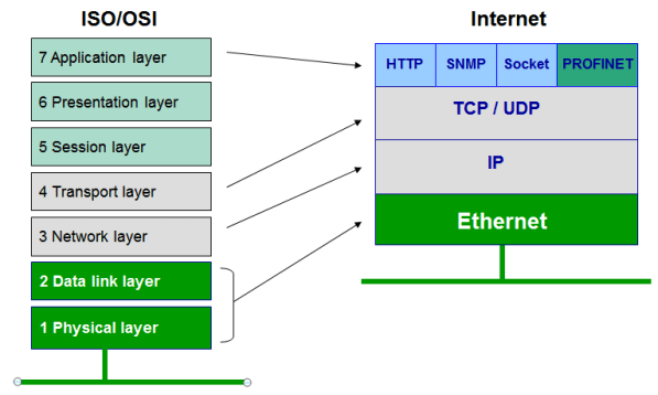
Ethernet is a protocol under IEEE 802.33 standard User Datagram Protocol (UDP) UDP is a connectionless transport protocol. I...